Evaluating diagnostic classification models

With Stan and measr

W. Jake Thompson, Ph.D.

Model evaluation

Absolute fit: How well does the model represent the observed data?
- Model-level
- Item-level
Relative fit: How do multiple models compare to each other?
Reliability: How consistent and accurate are the classifications?

Absolute model fit

Model-level absolute fit

Limited information indices based on parameter point estimates
- M₂ statistic (Liu et al., 2016)
Posterior predictive model checks (PPMCs)

fit_* functions are used for calculating absolute fit indices.

fit_m2(ecpe)

# A tibble: 1 × 8
     m2    df     pval  rmsea ci_lower ci_upper `90% CI`          srmsr
  <dbl> <int>    <dbl>  <dbl>    <dbl>    <dbl> <chr>             <dbl>
1  513.   325 1.33e-10 0.0141   0.0117   0.0163 [0.0117, 0.0163] 0.0319

add_fit() will add the fit index to the model object (and resave) to prevent unnecessary calculations in the future.

ecpe <- add_fit(ecpe, method = "m2")
measr_extract(ecpe, "m2")

# A tibble: 1 × 3
     m2    df     pval
  <dbl> <int>    <dbl>
1  513.   325 1.33e-10

Exercise 1

Open evaluation.Rmd and run the setup chunk.
Calculate the M₂ statistic for the MDM LCDM model using add_fit().
Extract the M₂ statistic. Does the model fit the data?

03:00

mdm_lcdm <- add_fit(mdm_lcdm, method = "m2")
measr_extract(mdm_lcdm, "m2")

# A tibble: 1 × 3
      m2    df  pval
   <dbl> <int> <dbl>
1 0.0306     1 0.861

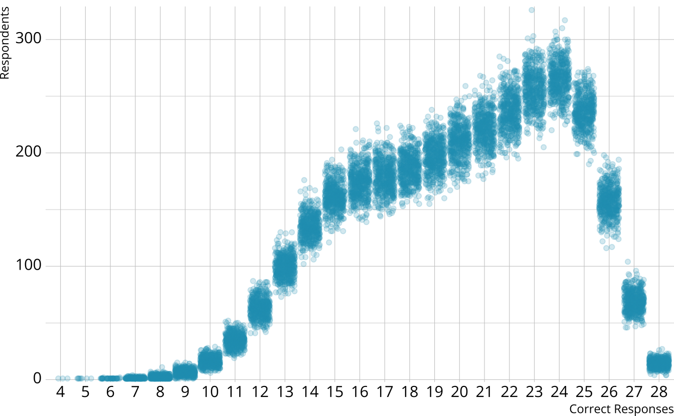
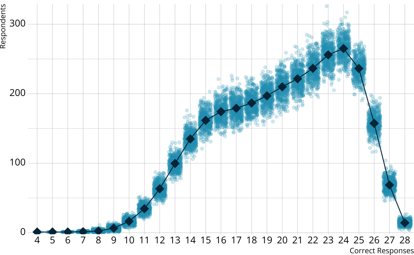
PPMC: Raw score distribution

For each iteration, calculate the total number of respondents at each score point

Calculate the expected number of respondents at each score point

Calculate the observed number of respondents at each score point

Scatter plot showing the number of respondents at each score point in each iteration.

Scatter plot showing the number of respondents at each score point in each iteration with the average number of respondents overlayed.

Scatter plot showing the number of respondents at each score point in each iteration with the average and observed number of respondents overlayed.

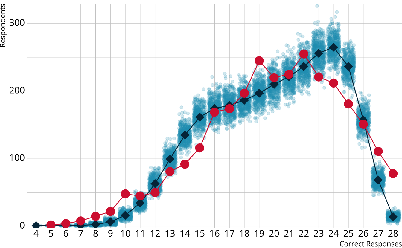
PPMC: \(\chi^2\)

Calculate a \(\chi^2\)-like statistic comparing the number of respondents at each score point in each iteration to the expectation

Calculate the \(\chi^2\) value comparing the observed data to the expectation

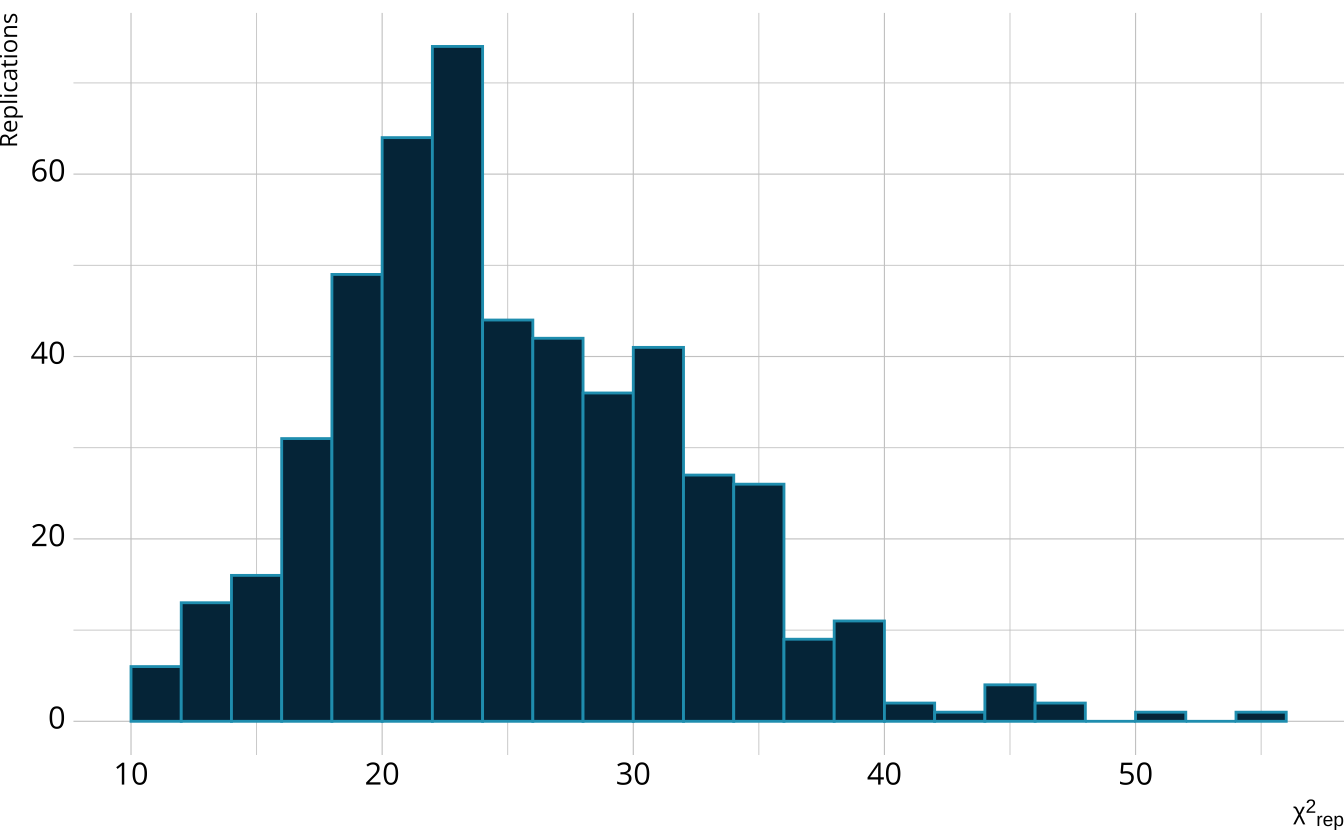
Histogram of the chi-square values from each iteration.

Histogram of the chi-square values from each iteration with a dashed vertical line indicating the value from the observed data.

PPMC: ppp

Calculate the proportion of iterations where the \(\chi^2\)-like statistic from replicated data set exceed the observed data statistic
- Posterior predictive p-value (ppp)

PPMCs with measr

One-time calculation
Save for future

fit_ppmc(ecpe, model_fit = "raw_score", item_fit = NULL)

$model_fit
$model_fit$raw_score
# A tibble: 1 × 5
  obs_chisq ppmc_mean `2.5%` `97.5%`   ppp
      <dbl>     <dbl>  <dbl>   <dbl> <dbl>
1     1004.      28.2   12.2    56.4     0

ecpe <- add_fit(ecpe, method = "ppmc", model_fit = "raw_score", item_fit = NULL)
measr_extract(ecpe, "ppmc_raw_score")

# A tibble: 1 × 5
  obs_chisq ppmc_mean `2.5%` `97.5%`   ppp
      <dbl>     <dbl>  <dbl>   <dbl> <dbl>
1      905.      26.9   13.0    54.7     0

Exercise 2

Calculate the raw score PPMC for the MDM LCDM
Does the model fit the observed data?

04:00

mdm_lcdm <- add_fit(mdm_lcdm, method = "ppmc", item_fit = NULL)
measr_extract(mdm_lcdm, "ppmc_raw_score")

# A tibble: 1 × 5
  obs_chisq ppmc_mean `2.5%` `97.5%`   ppp
      <dbl>     <dbl>  <dbl>   <dbl> <dbl>
1      3.36      6.90  0.736    20.3 0.726

Item-level fit

Diagnose problems with model-level
Identify particular items that may not be performing as expected
Identify potential dimensionality issues

Item-level fit with measr

Currently support two-measures of item-level fit using PPMCs:
- Conditional probability of each class providing a correct response (\(\pi\) matrix)
- Item pair odds ratios

Calculating item-level fit

ecpe <- add_fit(ecpe, method = "ppmc",
                item_fit = c("conditional_prob", "odds_ratio"))

Extracting item-level fit

Conditional probabilities
Odds ratios

measr_extract(ecpe, "ppmc_conditional_prob")

# A tibble: 224 × 7
   item  class   obs_cond_pval ppmc_mean `2.5%` `97.5%`   ppp
   <fct> <chr>           <dbl>     <dbl>  <dbl>   <dbl> <dbl>
 1 E1    [0,0,0]         0.701     0.694  0.662   0.723 0.324
 2 E1    [1,0,0]         0.782     0.798  0.712   0.905 0.597
 3 E1    [0,1,0]         1         0.810  0.757   0.865 0    
 4 E1    [0,0,1]         0.611     0.694  0.662   0.723 1    
 5 E1    [1,1,0]         0.996     0.930  0.909   0.952 0    
 6 E1    [1,0,1]         0.486     0.798  0.712   0.905 1    
 7 E1    [0,1,1]         0.831     0.810  0.757   0.865 0.222
 8 E1    [1,1,1]         0.926     0.930  0.909   0.952 0.654
 9 E2    [0,0,0]         0.741     0.739  0.708   0.767 0.455
10 E2    [1,0,0]         0.835     0.739  0.708   0.767 0    
# ℹ 214 more rows

measr_extract(ecpe, "ppmc_odds_ratio")

# A tibble: 378 × 7
   item_1 item_2 obs_or ppmc_mean `2.5%` `97.5%`    ppp
   <fct>  <fct>   <dbl>     <dbl>  <dbl>   <dbl>  <dbl>
 1 E1     E2       1.61      1.39   1.07    1.73 0.102 
 2 E1     E3       1.42      1.49   1.21    1.80 0.666 
 3 E1     E4       1.58      1.39   1.13    1.70 0.093 
 4 E1     E5       1.68      1.48   1.09    1.93 0.164 
 5 E1     E6       1.64      1.40   1.09    1.76 0.112 
 6 E1     E7       1.99      1.70   1.37    2.07 0.0505
 7 E1     E8       1.54      1.55   1.16    2.03 0.503 
 8 E1     E9       1.18      1.25   1.01    1.52 0.707 
 9 E1     E10      1.82      1.59   1.28    1.96 0.108 
10 E1     E11      1.61      1.64   1.32    2.01 0.566 
# ℹ 368 more rows

Flagging item-level fit

Conditional probabilities
Odds ratios

measr_extract(ecpe, "ppmc_conditional_prob_flags")

# A tibble: 105 × 7
   item  class   obs_cond_pval ppmc_mean `2.5%` `97.5%`   ppp
   <fct> <chr>           <dbl>     <dbl>  <dbl>   <dbl> <dbl>
 1 E1    [0,1,0]         1         0.810  0.757   0.865 0    
 2 E1    [0,0,1]         0.611     0.694  0.662   0.723 1    
 3 E1    [1,1,0]         0.996     0.930  0.909   0.952 0    
 4 E1    [1,0,1]         0.486     0.798  0.712   0.905 1    
 5 E2    [1,0,0]         0.835     0.739  0.708   0.767 0    
 6 E2    [0,1,0]         1         0.907  0.888   0.925 0    
 7 E2    [0,0,1]         0.694     0.739  0.708   0.767 0.998
 8 E2    [1,1,0]         0.975     0.907  0.888   0.925 0    
 9 E2    [1,0,1]         0.424     0.739  0.708   0.767 1    
10 E3    [0,1,0]         0.365     0.414  0.379   0.448 0.997
# ℹ 95 more rows

measr_extract(ecpe, "ppmc_odds_ratio_flags")

# A tibble: 80 × 7
   item_1 item_2 obs_or ppmc_mean `2.5%` `97.5%`    ppp
   <fct>  <fct>   <dbl>     <dbl>  <dbl>   <dbl>  <dbl>
 1 E1     E13      1.80      1.45   1.15    1.79 0.0215
 2 E1     E17      2.02      1.40   1.05    1.82 0.005 
 3 E1     E26      1.61      1.25   1.02    1.53 0.0075
 4 E1     E28      1.86      1.41   1.09    1.76 0.008 
 5 E2     E4       1.73      1.36   1.09    1.67 0.0055
 6 E2     E14      1.64      1.24   1.01    1.52 0.0025
 7 E2     E15      1.92      1.45   1.07    1.89 0.021 
 8 E3     E23      1.83      1.50   1.22    1.82 0.0205
 9 E3     E24      1.63      1.39   1.17    1.62 0.0205
10 E4     E5       2.81      2.09   1.58    2.67 0.012 
# ℹ 70 more rows

Patterns of item-level misfit

measr_extract(ecpe, "ppmc_conditional_prob_flags") |> 
  count(class, name = "flags") |> 
  left_join(measr_extract(ecpe, "strc_param"), by = join_by(class)) |> 
  arrange(desc(flags))

# A tibble: 8 × 3
  class   flags         estimate
  <chr>   <int>       <rvar[1d]>
1 [1,0,1]    21  0.0184 ± 0.0100
2 [0,1,0]    20  0.0164 ± 0.0109
3 [1,1,0]    19  0.0093 ± 0.0057
4 [1,0,0]    16  0.0118 ± 0.0063
5 [0,0,1]    14  0.1279 ± 0.0198
6 [0,1,1]     9  0.1730 ± 0.0203
7 [1,1,1]     4  0.3451 ± 0.0167
8 [0,0,0]     2  0.2981 ± 0.0165

Exercise 3

Calculate PPMCs for the conditional probabilities and odds ratios for the MDM model
What do the results tell us about the model?

05:00

mdm_lcdm <- add_fit(mdm_lcdm, method = "ppmc",
                    item_fit = c("conditional_prob", "odds_ratio"))

measr_extract(mdm_lcdm, "ppmc_conditional_prob_flags")

# A tibble: 0 × 7
# ℹ 7 variables: item <fct>, class <chr>, obs_cond_pval <dbl>, ppmc_mean <dbl>,
#   2.5% <dbl>, 97.5% <dbl>, ppp <dbl>

measr_extract(mdm_lcdm, "ppmc_odds_ratio_flags")

# A tibble: 0 × 7
# ℹ 7 variables: item_1 <fct>, item_2 <fct>, obs_or <dbl>, ppmc_mean <dbl>,
#   2.5% <dbl>, 97.5% <dbl>, ppp <dbl>

Relative model fit

Model comparisons

Doesn’t give us information whether or not a model fits the data, only compares competing models to each other
- Should be evaluated in conjunction with absolute model fit
Implemented with the loo package
- PSIS-LOO (Vehtari, 2017)
- WAIC (Watanabe, 2010)

Relative fit with measr

ecpe <- add_criterion(ecpe, criterion = c("loo", "waic"))

measr_extract(ecpe, "loo")


Computed from 2000 by 2922 log-likelihood matrix

         Estimate    SE
elpd_loo -42817.0 226.1
p_loo        76.6   0.8
looic     85634.0 452.2
------
Monte Carlo SE of elpd_loo is 0.2.

All Pareto k estimates are good (k < 0.5).
See help('pareto-k-diagnostic') for details.

Comparing models

First, we need another model to compare

ecpe_dina <- measr_dcm(
  data = ecpe_data, qmatrix = ecpe_qmatrix,
  resp_id = "resp_id", item_id = "item_id",
  type = "dina",
  method = "mcmc", backend = "cmdstanr",
  iter_warmup = 1000, iter_sampling = 500,
  chains = 4, parallel_chains = 4,
  file = "fits/ecpe-dina"
)

ecpe_dina <- add_criterion(ecpe_dina, criterion = "loo")

`loo_compare()`

loo_compare(ecpe, ecpe_dina, criterion = "loo",
            model_names = c("lcdm", "dina"))

     elpd_diff se_diff
lcdm    0.0       0.0 
dina -808.6      39.3

LCDM is the preferred model
- Preferred does not imply “good”
- Remember, the LCDM showed poor absolute fit
Difference is much larger than the standard error of the difference

Exercise 4

Estimate a DINA model for the MDM data
Add PSIS-LOO and WAIC criteria to both the LCDM and DINA models for the MDM data
Use loo_compare() to compare the LCDM and DINA models
- What do the findings tell us?
- Can you explain the results?

05:00

Estimate DINA model
Add criterion
Compare models

mdm_dina <- measr_dcm(
  data = mdm_data, qmatrix = mdm_qmatrix,
  resp_id = "respondent", item_id = "item",
  type = "dina",
  method = "mcmc", backend = "rstan",
  warmup = 1000, iter = 1500, chains = 2,
  file = "fits/mdm-dina"
)

mdm_lcdm <- add_criterion(mdm_lcdm, criterion = c("loo", "waic"))
mdm_dina <- add_criterion(mdm_dina, criterion = c("loo", "waic"))

loo_compare(mdm_lcdm, mdm_dina, criterion = "loo")

         elpd_diff se_diff
mdm_lcdm  0.0       0.0   
mdm_dina -0.2       2.5

loo_compare(mdm_lcdm, mdm_dina, criterion = "waic")

         elpd_diff se_diff
mdm_lcdm  0.0       0.0   
mdm_dina -0.2       2.5

Reliability

Reliability methods

Reporting reliability depends on how results are estimated and reported
Reliability for:
- Profile-level classification
- Attribute-level classification
- Attribute-level probability of proficiency

Reliability with measr

One-time calculation
Save for future

reliability(ecpe)

$pattern_reliability
      p_a       p_c 
0.7390218 0.6637287 

$map_reliability
$map_reliability$accuracy
# A tibble: 3 × 8
  attribute         acc lambda_a kappa_a youden_a tetra_a  tp_a  tn_a
  <chr>           <dbl>    <dbl>   <dbl>    <dbl>   <dbl> <dbl> <dbl>
1 morphosyntactic 0.896    0.729   0.787    0.775   0.942 0.851 0.924
2 cohesive        0.852    0.675   0.704    0.699   0.892 0.877 0.822
3 lexical         0.916    0.750   0.610    0.802   0.959 0.947 0.855

$map_reliability$consistency
# A tibble: 3 × 10
  attribute       consist lambda_c kappa_c youden_c tetra_c  tp_c  tn_c gammak
  <chr>             <dbl>    <dbl>   <dbl>    <dbl>   <dbl> <dbl> <dbl>  <dbl>
1 morphosyntactic   0.834    0.557   0.685    0.646   0.853 0.778 0.868  0.852
2 cohesive          0.806    0.562   0.681    0.607   0.817 0.826 0.781  0.789
3 lexical           0.856    0.552   0.626    0.670   0.875 0.894 0.776  0.880
# ℹ 1 more variable: pc_prime <dbl>


$eap_reliability
# A tibble: 3 × 5
  attribute       rho_pf rho_bs rho_i rho_tb
  <chr>            <dbl>  <dbl> <dbl>  <dbl>
1 morphosyntactic  0.734  0.687 0.573  0.884
2 cohesive         0.728  0.575 0.506  0.785
3 lexical          0.758  0.730 0.587  0.915

ecpe <- add_reliability(ecpe)

Profile-level classification

Profile-level probabilities
Profile-level classifications
Profile reliability

measr_extract(ecpe, "class_prob")

# A tibble: 2,922 × 9
   resp_id `[0,0,0]` `[1,0,0]` `[0,1,0]` `[0,0,1]` `[1,1,0]` `[1,0,1]` `[0,1,1]`
   <fct>       <dbl>     <dbl>     <dbl>     <dbl>     <dbl>     <dbl>     <dbl>
 1 1         7.70e-6   9.83e-5   5.11e-7  0.00131  0.0000875  0.0436     0.00208
 2 2         5.85e-6   7.43e-5   2.00e-7  0.00306  0.0000344  0.0974     0.00196
 3 3         5.63e-6   1.67e-5   1.73e-6  0.00211  0.0000701  0.00970    0.0154 
 4 4         3.21e-7   4.06e-6   9.79e-8  0.000296 0.0000167  0.00985    0.00215
 5 5         1.17e-3   8.30e-3   3.57e-4  0.00127  0.0353     0.00933    0.00921
 6 6         2.97e-6   1.59e-5   9.08e-7  0.000912 0.0000651  0.00980    0.00663
 7 7         2.97e-6   1.59e-5   9.08e-7  0.000912 0.0000651  0.00980    0.00663
 8 8         3.73e-2   8.52e-5   1.34e-3  0.518    0.0000259  0.000586   0.439  
 9 9         6.55e-5   2.02e-4   2.00e-5  0.00657  0.000921   0.00933    0.0479 
10 10        4.05e-1   4.15e-1   3.58e-3  0.0379   0.0611     0.0180     0.00780
# ℹ 2,912 more rows
# ℹ 1 more variable: `[1,1,1]` <dbl>

measr_extract(ecpe, "class_prob") |> 
  pivot_longer(-resp_id,
               names_to = "profile",
               values_to = "prob") |> 
  slice_max(order_by = prob,
            by = resp_id)

# A tibble: 2,922 × 3
   resp_id profile  prob
   <fct>   <chr>   <dbl>
 1 1       [1,1,1] 0.953
 2 2       [1,1,1] 0.897
 3 3       [1,1,1] 0.973
 4 4       [1,1,1] 0.988
 5 5       [1,1,1] 0.935
 6 6       [1,1,1] 0.983
 7 7       [1,1,1] 0.983
 8 8       [0,0,1] 0.518
 9 9       [1,1,1] 0.935
10 10      [1,0,0] 0.415
# ℹ 2,912 more rows

measr_extract(ecpe, "pattern_reliability")

# A tibble: 1 × 2
  accuracy consistency
     <dbl>       <dbl>
1    0.739       0.664

Estimating classification consistency and accuracy for cognitive diagnostic assessment (Cui et al., 2012)

Attribute-level classification

Attribute-level probabilities
Attribute-level classifications
Classification reliability

measr_extract(ecpe, "attribute_prob")

# A tibble: 2,922 × 4
   resp_id morphosyntactic cohesive lexical
   <fct>             <dbl>    <dbl>   <dbl>
 1 1               0.997      0.955   1.00 
 2 2               0.995      0.899   1.00 
 3 3               0.983      0.988   1.00 
 4 4               0.998      0.990   1.00 
 5 5               0.988      0.980   0.955
 6 6               0.992      0.989   1.00 
 7 7               0.992      0.989   1.00 
 8 8               0.00436    0.444   0.961
 9 9               0.945      0.984   0.999
10 10              0.545      0.123   0.115
# ℹ 2,912 more rows

measr_extract(ecpe, "attribute_prob") |> 
  mutate(
    across(
      where(is.double),
      ~case_when(.x > 0.5 ~ 1L,
                 TRUE ~ 0L)
    )
  )

# A tibble: 2,922 × 4
   resp_id morphosyntactic cohesive lexical
   <fct>             <int>    <int>   <int>
 1 1                     1        1       1
 2 2                     1        1       1
 3 3                     1        1       1
 4 4                     1        1       1
 5 5                     1        1       1
 6 6                     1        1       1
 7 7                     1        1       1
 8 8                     0        0       1
 9 9                     1        1       1
10 10                    1        0       0
# ℹ 2,912 more rows

measr_extract(ecpe, "classification_reliability")

# A tibble: 3 × 3
  attribute       accuracy consistency
  <chr>              <dbl>       <dbl>
1 morphosyntactic    0.896       0.834
2 cohesive           0.852       0.806
3 lexical            0.916       0.856

Measures of agreement to assess attribute-level classification accuracy and consistency for cognitive diagnostic assessments (Johnson & Sinharay, 2018)

Attribute-level probabilities

Attribute-level probabilities
Probability reliability

measr_extract(ecpe, "attribute_prob")

# A tibble: 2,922 × 4
   resp_id morphosyntactic cohesive lexical
   <fct>             <dbl>    <dbl>   <dbl>
 1 1               0.997      0.955   1.00 
 2 2               0.995      0.899   1.00 
 3 3               0.983      0.988   1.00 
 4 4               0.998      0.990   1.00 
 5 5               0.988      0.980   0.955
 6 6               0.992      0.989   1.00 
 7 7               0.992      0.989   1.00 
 8 8               0.00436    0.444   0.961
 9 9               0.945      0.984   0.999
10 10              0.545      0.123   0.115
# ℹ 2,912 more rows

measr_extract(ecpe, "probability_reliability")

# A tibble: 3 × 2
  attribute       informational
  <chr>                   <dbl>
1 morphosyntactic         0.573
2 cohesive                0.506
3 lexical                 0.587

The reliability of the posterior probability of skill attainment in diagnostic classification models (Johnson & Sinharay, 2020)

Exercise 5

Add reliability information to the MDM LCDM and DINA models
Examine the attribute classification indices for both models

04:00

Calculate reliability
Compare reliability

mdm_lcdm <- add_reliability(mdm_lcdm)
mdm_dina <- add_reliability(mdm_dina)

measr_extract(mdm_lcdm, "classification_reliability")

# A tibble: 1 × 3
  attribute      accuracy consistency
  <chr>             <dbl>       <dbl>
1 multiplication    0.898       0.819

measr_extract(mdm_dina, "classification_reliability")

# A tibble: 1 × 3
  attribute      accuracy consistency
  <chr>             <dbl>       <dbl>
1 multiplication    0.905       0.831

Evaluating diagnostic classification models

With Stan and measr

https://stancon2023.measr.info